Search algorithms aren’t new, but some are just better at scaling. That’s where HNSW comes in. If you’ve ever wondered how a system can find the right match in millions of options and still respond quickly, HNSW is part of that answer. Built for approximate nearest neighbor (ANN) search, it blends speed with accuracy in a way that traditional brute-force approaches can’t handle. It works behind the scenes in everything from recommendation engines to search functions in machine learning applications.

So, what exactly is it, and how does it manage to perform so well? Let’s take a look.

What Is HNSW and Why It Works

At its core, HNSW stands for Hierarchical Navigable Small World. It's a graph-based algorithm that builds on the idea of connecting data points not just randomly but in a structured way that makes traversal fast. The "small world" part isn't just a catchy phrase. It refers to the small-world network principle—most nodes (or data points) can be reached in a few steps because of how the network is built.

Imagine trying to find the closest airport to a city. Instead of checking every single city and then choosing the closest, HNSW allows you to take a shortcut. It connects points in such a way that the system can jump to a neighborhood of likely options and then fine-tune from there. The benefit? You get a good enough answer fast, without digging through the entire pile.

This makes it ideal for cases where time matters and the result doesn't need to be exact but close enough—think voice recognition, image search, or similarity-based recommendations.

How HNSW Is Structured

Multi-layer Graph Design

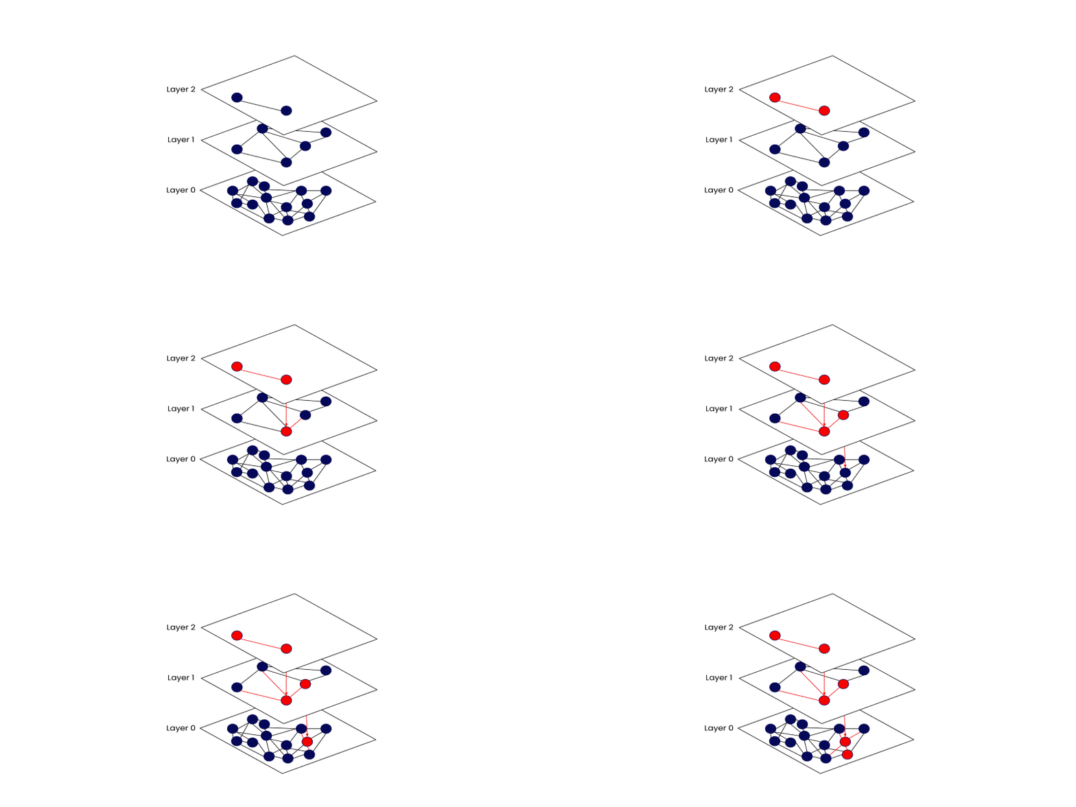
The structure looks like a set of floors in a building. Each higher layer has fewer nodes but longer connections. The top layer offers a broad view, helping the system make big jumps across the dataset. As the search moves lower, it becomes more focused, narrowing down to more detailed neighborhoods. The lowest layer contains all the points and provides the closest matches.

This layered approach reduces the number of steps needed to find a nearby point. You start at the top, make large leaps toward the target region, and then gradually refine the search as you move down. Think of it as zooming in on a map. You start with the general region, then move street by street until you get to the front door.

2. Neighbor Selection and Connection Rules

When a new point is added to the graph, the system doesn’t just plug it in randomly. It evaluates its similarity to existing points and forms connections based on distance. But there’s a limit to how many links one point can have. This keeps the network from becoming too cluttered, which could slow things down.

The algorithm uses a heuristic that tries to avoid forming connections between points that are already close to one another. Instead, it aims for diversity in the links, which helps maintain that small-world efficiency.

3. Search Process: Greedy but Smart

The search starts at the top layer and makes decisions greedily—it always moves to the neighbor closest to the query. Once it can't get any closer to the current level, it drops down to the next. By the time it reaches the bottom, the search zone is already narrowed down to the most relevant cluster of points.

This method might sound simple, but its efficiency is what makes it powerful. It skips over vast portions of the dataset while still finding high-quality matches.

Steps to Build and Use an HNSW Graph

Setting up HNSW is more than just calling a function. There’s a process behind it, and understanding each step helps make the most of its strengths.

Step 1: Initialize Parameters

Before anything else, you need to set parameters. Two key ones are M and efConstruction.

• M controls how many connections each node can have. A higher value means more links, which can improve accuracy but will require more memory.
• efConstruction affects the quality of the graph during the build phase. A higher value means more candidates are considered when adding a new point.

Choosing these settings depends on the balance you want between speed, memory, and precision.

Step 2: Insert Data Points

Each point is added one at a time. For each new point, the system picks a random layer for it. The higher the layer, the fewer points exist there, which helps in keeping the upper layers lean and fast. Then, it performs a search from the top layer down, finding the best neighbors at each level.

At each layer, the system connects the point to nearby nodes, following the neighbor selection rules mentioned earlier. These connections allow future searches to use this point as part of the network.

Step 3: Set ef for Runtime Search

The ef parameter comes into play during the search. It defines how many candidates are explored before the system decides on the final neighbors. A higher ef increases recall (getting closer to the best match) but slows the query slightly. It's a trade-off between quality and time.

Once the graph is built, changing ef doesn’t require rebuilding—it just affects search performance at runtime.

Step 4: Run Queries

With the graph in place and ef tuned, running a query involves finding the closest vector or data point to your input. The algorithm begins at the highest layer, navigates through the graph greedily, and refines the result as it moves down.

The final output is a list of nearest neighbors, usually returned within milliseconds, even for very large datasets.

Why HNSW Became the Go-To for ANN

There are other ANN algorithms like KD-Trees, Ball Trees, and LSH, but HNSW has something most others don't: consistently high performance on large, high-dimensional datasets.

KD-Trees and Ball Trees work well in low dimensions but don’t scale. LSH handles some higher-dimensional data, but often with less precision. HNSW, on the other hand, scales well and maintains good recall across a wide range of tasks. That’s why it’s widely used in open-source libraries like FAISS and hnswlib.

It handles both high-throughput and low-latency requirements, which is exactly what modern applications need.

Closing Thoughts

HNSW does a lot with relatively simple ideas: structured layering, smart connections, and greedy traversal. The result is a graph that balances speed and quality without needing brute force. Whether you’re building a search feature for a product catalog or working with machine learning models that need quick vector comparisons, this algorithm holds up.